Data Visualization

Data Skills for Psychology — Module 4

Welcome!

These slides are adapted from Applied Data Skills Ch. 3.

Today’s Goals

By the end of this class, you will be able to:

• Describe the layered grammar of graphics behind {ggplot2}
• Build a plot layer by layer: data, mapping, geoms, scales, themes
• Pick an appropriate plot type for categorical vs. continuous data
• Customize axes, labels, colours, and themes
• Make your plots easier to read using jitter and facets
• Save plots with ggsave()

Setup

Make sure you have these packages loaded:

library(tidyverse)   # readr, dplyr, ggplot2, etc.
library(patchwork)   # combine plots side-by-side
library(ggthemes)    # extra themes

Tip

If you haven’t installed patchwork or ggthemes yet, run in the Console:
install.packages(c("patchwork", "ggthemes"))

You only need to do this once!

Our Dataset

We’ll use data from the World Bank’s Poverty and Inequality Platform. Load it from the web:

pip <- read_csv("https://raw.githubusercontent.com/PsyTeachR/ads-v3/refs/heads/master/data/pip_gini_welfare_2010.csv")

Each row is one country in 2010. Key columns:

• region_name, region_code — world region
• country_name, country_code — country
• gini — inequality (0 = perfect equality, 1 = complete inequality)
• welfare_mean — mean welfare per capita
• welfare_median — median welfare per capita

The Grammar of Graphics

Plots are Built in Layers

{ggplot2} uses a layered grammar of graphics: plots are built up one piece at a time.

Think of it like building a presentation slide — each layer sits on top of the last:

1. A blank canvas
2. Variables mapped to axes
3. A geom (the shape that represents your data)
4. Maybe more geoms on top
5. Axis tweaks and labels
6. A theme

Each layer is independently customizable — and you add them with +.

Set a Default Theme

The book uses the black-and-white theme, not the default grey one. Add this to your setup chunk:

theme_set(theme_bw())   # applies to every plot you make

You can always override it on a per-plot basis — but this keeps things consistent.

Building a Plot, Layer by Layer

Layer 1: A Blank Plot

Every plot starts with ggplot() and a data table:

ggplot(data = pip)

That’s it — a blank grey box. No variables yet, so there’s nothing to draw.

Layer 2: Mapping Variables

Use aes() (aesthetic mapping) to tell ggplot which columns go where:

ggplot(data = pip,
       mapping = aes(x = gini, y = welfare_mean))

Now the axes exist, but there’s still nothing drawn — we haven’t told it how to represent the data.

Note

In practice, almost everyone drops the argument names and writes the code more like this:

ggplot(pip, aes(x = gini, y = welfare_mean))

Layer 3: Add a Geom

Geoms are the shapes that represent your data — their functions all start with geom_. Add one with +:

ggplot(pip, aes(x = gini, y = welfare_mean)) +
  geom_point()

Watch the +!

The + has to be at the end of the previous line, not at the start of the next one. If you write + geom_point() on its own line, you’ll get an error.

Multiple Geoms

You can stack geoms — order matters (later layers draw on top):

# boxplot with points on top
ggplot(pip, aes(x = region_name, y = welfare_mean)) +
  geom_boxplot(width = .2) +
  geom_jitter(width = .2) +
  coord_flip()

# points behind the boxplot
ggplot(pip, aes(x = region_name, y = welfare_mean)) +
  geom_jitter(width = .2) +
  geom_boxplot(width = .2) +
  coord_flip()

Activity: Your First Plot

Try it!

1. Load the pip data with read_csv() (see the Setup slide).
2. Run theme_set(theme_bw()).
3. Make a scatterplot of gini on x and welfare_mean on y. Which geom should you use?
4. Bonus: Add a second geom — geom_smooth(method = "lm", formula = y ~ x) — to show a trendline.

Common Geoms

There are a lot of different geoms, but these are ones that you’ll see most in this class:

• geom_point
• geom_jitter
• geom_boxplot
• geom_line
• geom_histogram
• geom_errorbar
• geom_smooth

Styling Geoms

Styling the Whole Geom

To change how all points (or lines, or bars) look, set arguments inside the geom — not inside aes():

ggplot(pip, aes(x = gini, y = welfare_mean)) +
  geom_point(colour = "dodgerblue",
             alpha = 0.2,      # 20% transparency
             shape = 18,       # solid diamond
             size = 2) +
  geom_smooth(method = lm,
              formula = y ~ x,
              colour = "navy",
              linetype = 3)    # dotted line

Style by Category

When you want the style to represent a variable, put it inside aes() instead:

# colour points by region
ggplot(pip, aes(x = gini, y = welfare_mean,
                colour = region_code)) +
  geom_point(alpha = 0.6)

The golden rule

• Inside aes() → the aesthetic represents data
• Outside aes() (in the geom) → the aesthetic is a fixed style

A note on ggplot syntax

If you find yourself getting tripped up by the syntax for ggplot, don’t worry. This is normal!

It is common for researchers to find examples of what they want online, and then tweak the examples to fit their project.

Picking the Right Plot

Match the Plot to the Data

Different kinds of data call for different plots. We’ll walk through the most common cases:

• Counts of categories → bar / column plot
• One continuous variable → histogram
• Continuous variable by group → violin, boxplot, combo
• Two continuous variables → scatterplot + trendline

The ggplot2 cheat sheet is a great quick reference.

Counting Categories: geom_bar()

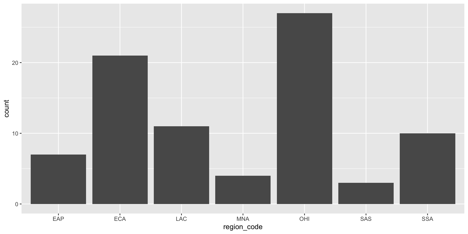
geom_bar() counts rows per category — only needs an x aesthetic:

ggplot(pip, aes(x = region_code)) +
  geom_bar()

Add fill inside aes() to colour bars by category:

ggplot(pip, aes(x = region_code, fill = region_code)) +
  geom_bar()

geom_col() for Pre-computed Counts

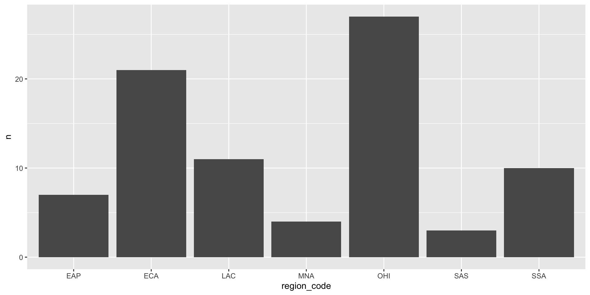
If your data already has a count column, use geom_col() (which needs both x and y):

count_data <- count(pip, region_code, sort = TRUE)

ggplot(count_data, aes(x = region_code, y = n)) +
  geom_col()

Use fct_reorder() to sort bars by size:

ggplot(count_data,
       aes(x = fct_reorder(region_code, n), y = n)) +
  geom_col() +
  labs(x = "Region")

One Continuous Variable

Histograms

geom_histogram() splits a continuous variable into bins and counts each bin:

ggplot(pip, aes(x = welfare_mean)) +
  geom_histogram(binwidth = 5, boundary = 0,
                 fill = "white", color = "black")

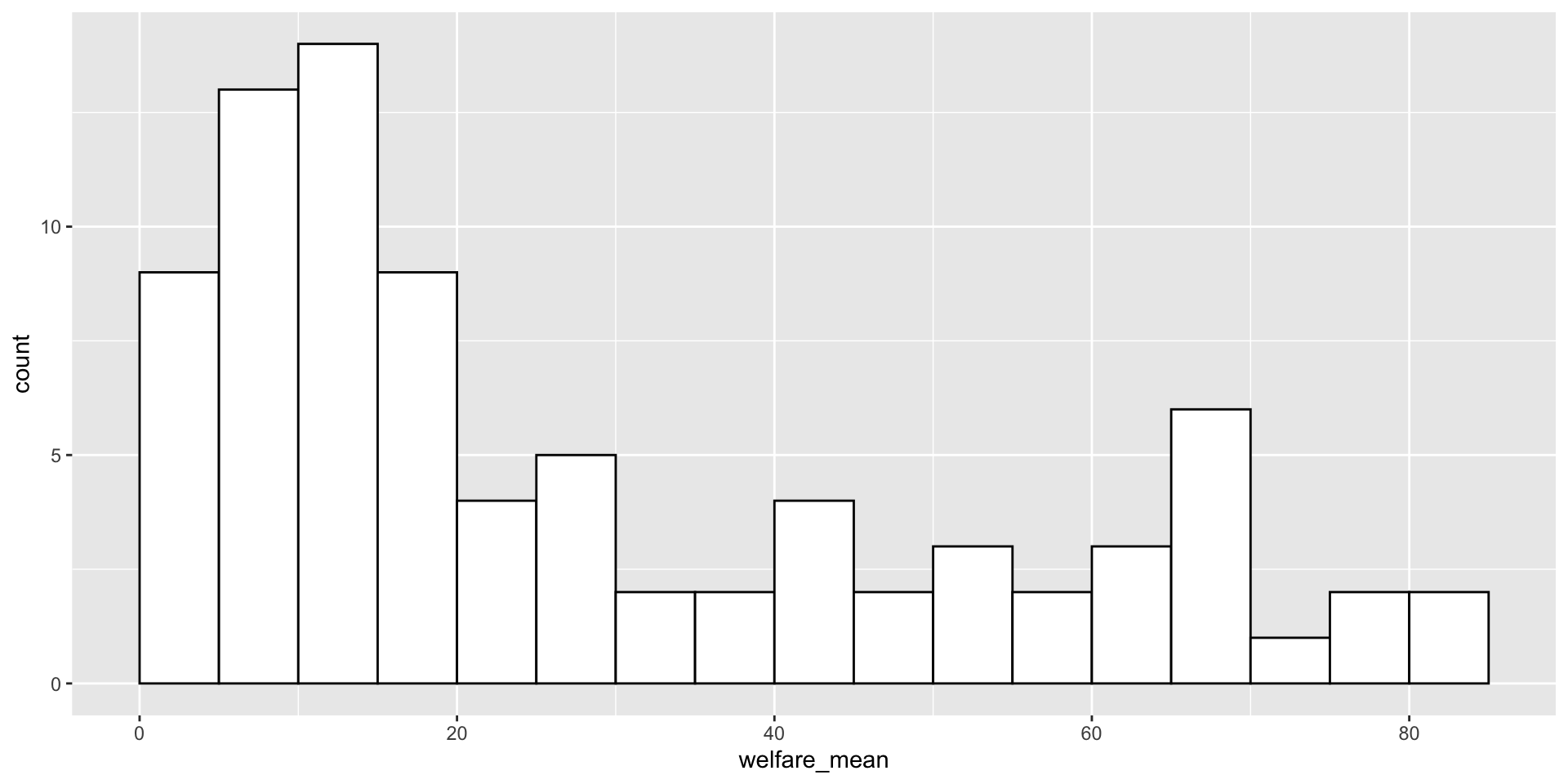
Always set binwidth or bins — the default usually isn’t what you want.

Grouped Continuous: Violin Plot

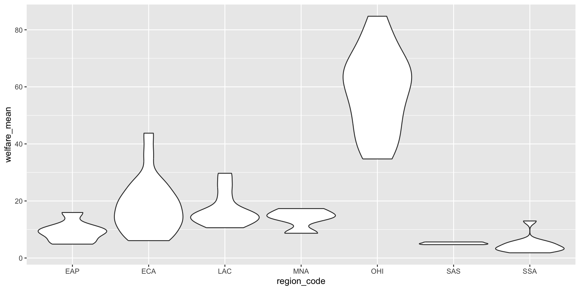
Violin plots show the shape of a distribution for each group:

ggplot(pip, aes(x = region_code, y = welfare_mean)) +
  geom_violin(scale = "width")

Grouped Continuous: Boxplot

Boxplots show summary statistics, not shape:

ggplot(pip, aes(x = region_code, y = welfare_mean)) +
  geom_boxplot()

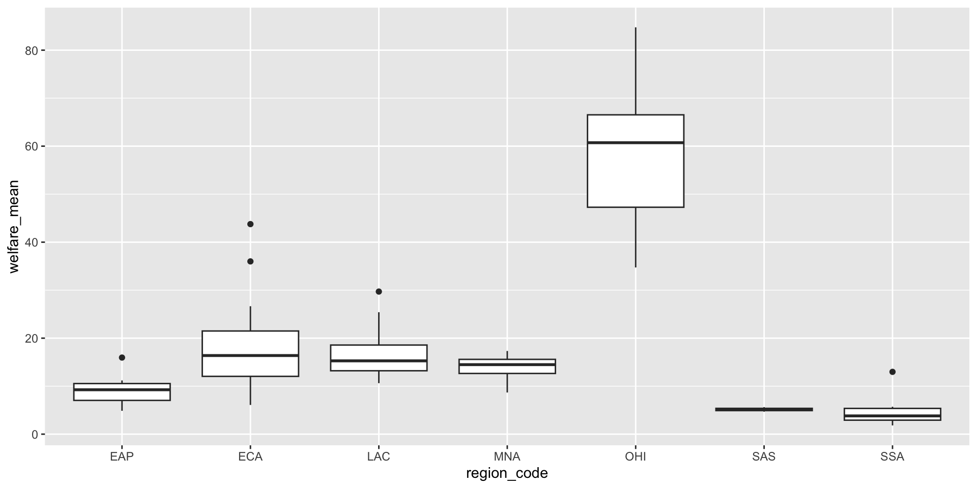
What’s in a boxplot:

• The middle line is the median (50th percentile)
• The box goes from the 25th to 75th percentile
• The whiskers extend 1.5× the box height
• The points are outliers

Combo: Violin + Boxplot + Mean

You can layer geoms to show shape, summary, and mean all at once:

ggplot(pip, aes(x = region_code, y = welfare_mean,
                fill = region_code)) +
  geom_violin(alpha = 0.4, scale = "width") +
  geom_boxplot(width = 0.25, fill = "white",
               alpha = 0.75, outlier.alpha = 0) +
  stat_summary(fun = mean, geom = "point",
               size = 2, shape = 18) +
  guides(fill = "none") +
  labs(x = "Region", y = "Mean Welfare per Capita")

Activity: Compare Distributions

Try it!

Using the pip data:

1. Make a histogram of gini (binwidth around 0.02 is a reasonable start).
2. Make a violin plot of gini by region_code.
3. Make a boxplot of the same thing.
4. Bonus: Which plot best shows that some regions have narrow inequality distributions while others are broad?

Two Continuous Variables

Scatterplot

geom_point() is the workhorse for two continuous variables:

ggplot(pip, aes(x = gini, y = welfare_mean)) +
  geom_point()

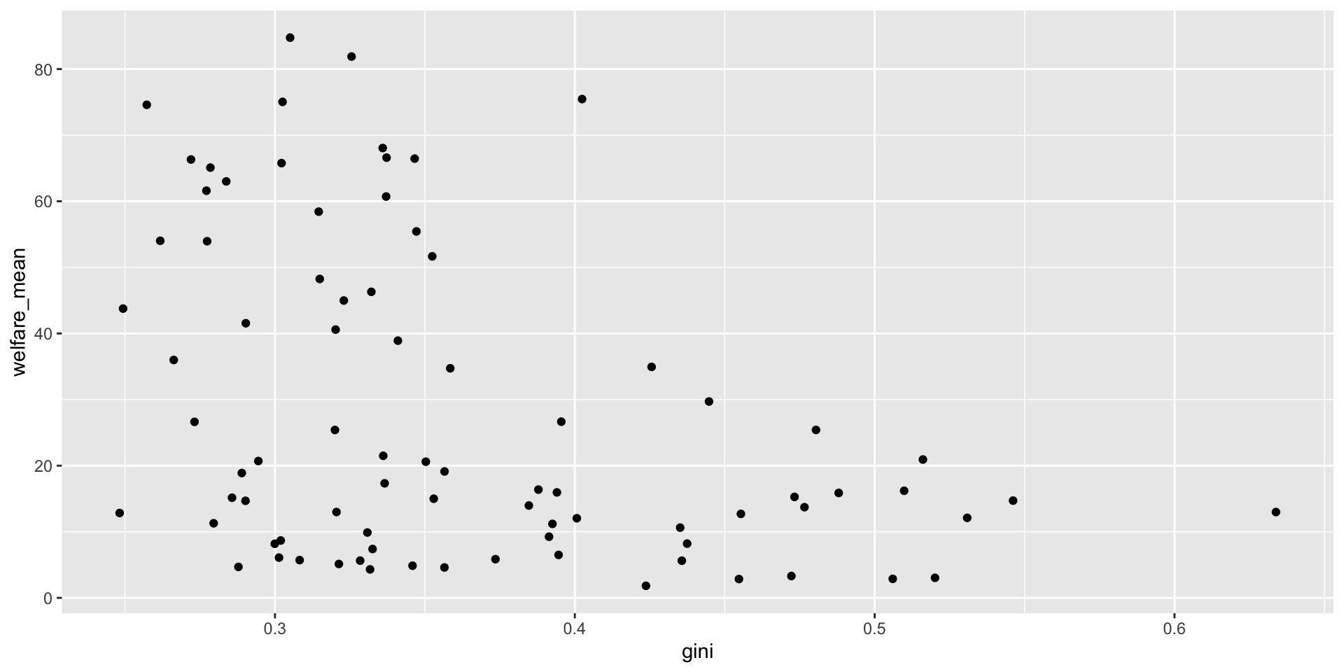
A good rule of thumb: put the cause (or predictor) on the x-axis and the effect (or outcome) on the y-axis.

Adding a Trendline

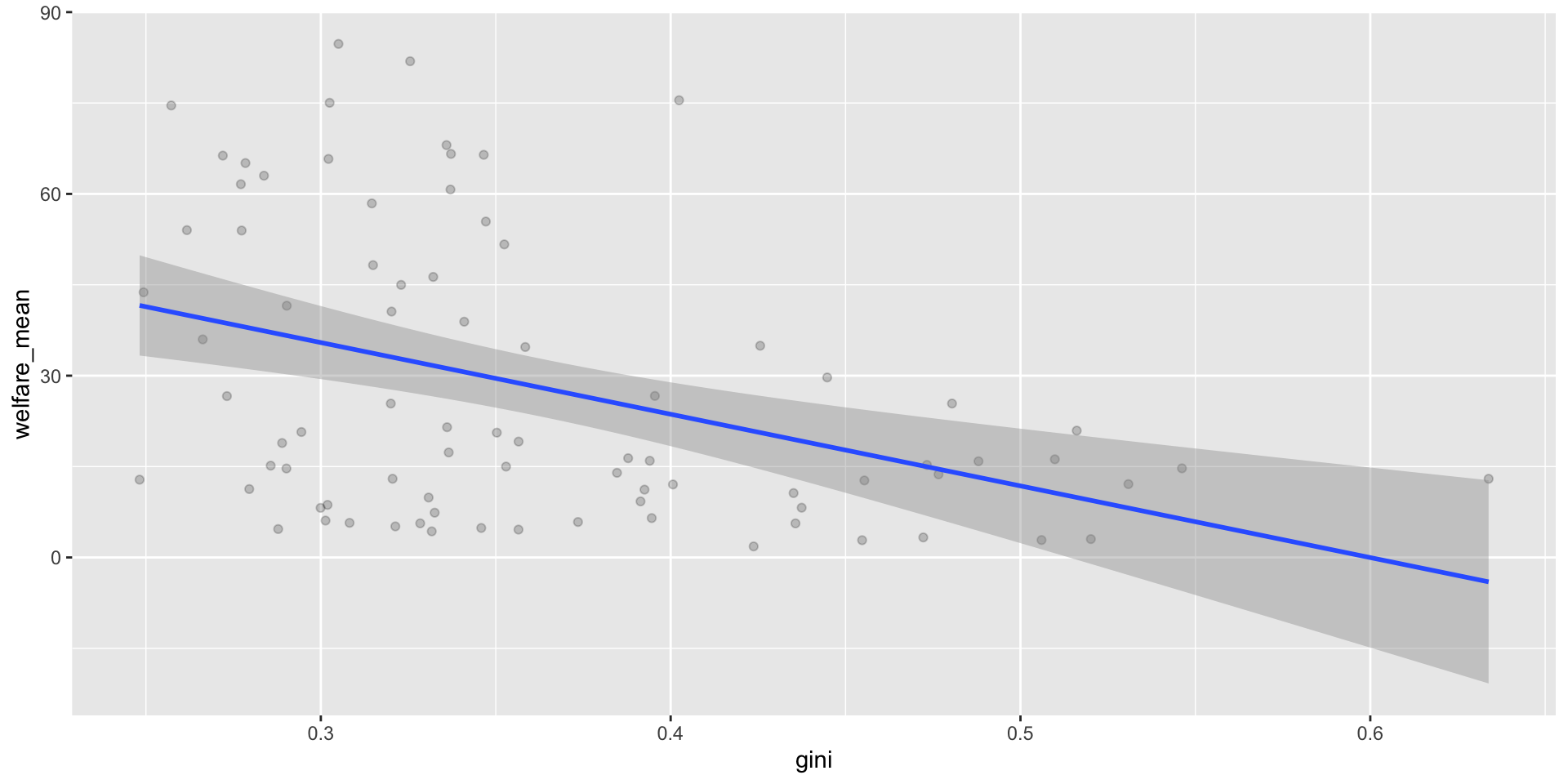
geom_smooth() fits a line through the data. The shaded ribbon is the confidence interval.

ggplot(pip, aes(x = gini, y = welfare_mean)) +
  geom_point(alpha = 0.2) +
  geom_smooth(method = lm, formula = y ~ x)   # linear

Other trendline options

• method = loess — flexible, wavy line (default for small data)
• method = lm, formula = y ~ x + I(x^2) — quadratic (one bend)
• Add se = FALSE to hide the confidence ribbon

Axes and Scales

The scale_ Family

scale_ functions control how each aesthetic maps to the plot. Match the function to the data type:

Data type	x-axis	y-axis
Continuous	scale_x_continuous()	scale_y_continuous()
Categorical	scale_x_discrete()	scale_y_discrete()

Axis Limits

To zoom in without dropping data, use coord_cartesian():

ggplot(pip, aes(x = gini, y = welfare_mean)) +
  geom_point(alpha = 0.2) +
  coord_cartesian(ylim = c(0, 100))

Warning

Setting limits inside scale_ actually drops data outside the range. This matters for things like boxplots and violins! Use coord_cartesian() to just zoom.

Themes and Labels

Built-in Themes

{ggplot2} ships with several themes; {ggthemes} adds many more:

ggplot(pip, aes(x = gini, y = welfare_mean)) +
  geom_point(alpha = 0.2) +
  theme_light(base_size = 11)   # font size in points

Some favourites to try: theme_minimal(), theme_bw(), theme_classic(), ggthemes::theme_gdocs().

Theme Tweaks

theme() lets you override any theme element. Use element_blank() to remove something:

ggplot(pip, aes(x = gini, y = welfare_mean)) +
  geom_point(alpha = 0.2) +
  theme_light(base_size = 11) +
  theme(plot.background = element_blank())   # remove outer border

Check ?theme to see the (large!) list of things you can tweak.

Labels with labs()

labs() adds a title, subtitle, caption, and axis labels all at once:

ggplot(pip, aes(x = gini, y = welfare_mean)) +
  geom_point(alpha = 0.2) +
  labs(title = "Inequality vs. welfare across regions",
       subtitle = "Data from 2010",
       x = "Gini Index",
       y = "Mean Welfare per Capita",
       caption = "Source: World Bank PIP")

Activity: Style a Plot

Try it!

Starting from your scatterplot:

1. Add alpha = 0.3 to geom_point() so the points are transparent.
2. Use scale_x_continuous() and scale_y_continuous() to add nicer axis labels.
3. Apply a theme you like (try theme_minimal() or theme_light()).
4. Use labs() to add a title, subtitle, and caption.
5. Bonus: Colour the points by region_code.

Saving Plots

ggsave()

ggsave() saves the last plot you made by default:

ggsave("my_plot.png", width = 5, height = 7)

Or save a plot you stored in an object:

box <- ggplot(pip, aes(x = region_name, y = gini)) +
  geom_boxplot()

ggsave("box_plot.jpg", plot = box, width = 7, height = 7)

The file type comes from the extension (.png, .jpg, .pdf, .svg, …). Default units are inches, but you can pass units = "cm" or "mm".

Dealing with Overplotting

The Problem

When lots of points pile up on the same spot, you can’t see what’s there:

# imagine simdat with 10,000 rows and ratings of 1–5
ggplot(simdat, aes(x = score, y = rating)) +
  geom_point()

Every rating is only 1, 2, 3, 4, or 5 — so all points squash onto 5 horizontal lines.

Fix 1: Jitter

geom_jitter() nudges each point a random tiny amount:

ggplot(simdat, aes(x = score, y = rating)) +
  geom_jitter(height = 0.2, width = 0, alpha = 0.1)

• height / width — how far to nudge (in data units)
• alpha — transparency, so overlapping points add up visibly

Fix 2: Facets

facet_wrap() breaks the plot into small multiples — one panel per category:

ggplot(simdat, aes(x = score)) +
  geom_histogram(binwidth = 5, boundary = 0,
                 fill = "dodgerblue", color = "black") +
  facet_wrap(~ rating, ncol = 1, labeller = label_both)

Read ~ rating as “by rating”. label_both adds both the variable name and its value to each panel.

Putting It All Together

A Publication-Ready Plot

Start simple, add layers until you’re happy:

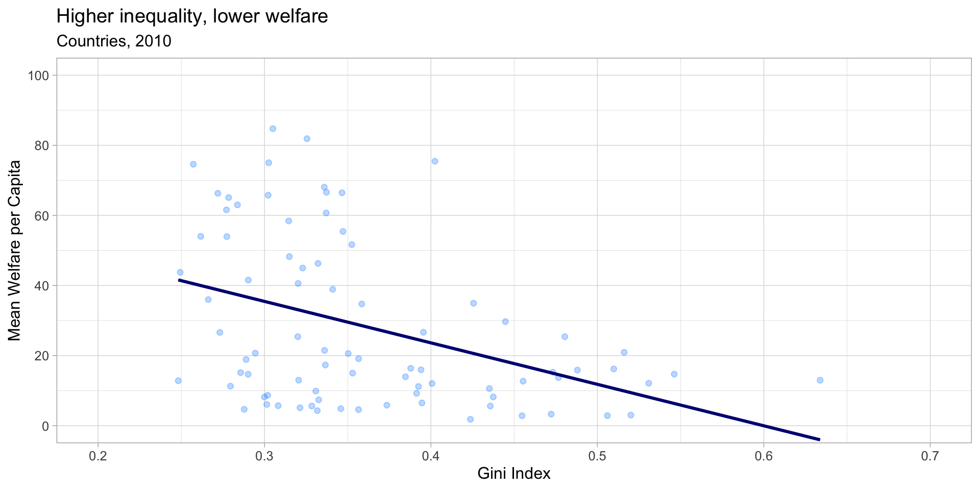
ggplot(pip, aes(x = gini, y = welfare_mean)) +
  geom_point(colour = "dodgerblue", alpha = 0.3) +
  geom_smooth(method = lm, formula = y ~ x,
              colour = "navy", se = FALSE) +
  scale_x_continuous(name = "Gini Index",
                     breaks = seq(0, 1, .1)) +
  scale_y_continuous(name = "Mean Welfare per Capita",
                     breaks = seq(0, 100, 20)) +
  coord_cartesian(xlim = c(.2, .7), ylim = c(0, 100)) +
  theme_light(base_size = 12) +
  theme(plot.background = element_blank()) +
  labs(title = "Higher inequality, lower welfare",
       subtitle = "Countries, 2010")

Build these plots one layer at a time — render at each step. It’s much easier to find the broken layer that way.

A Publication-Ready Plot

Wrapping Up

Key Takeaways

• ggplot() + aes() + geom_*() — the three minimum ingredients
• Inside aes() → represents data; outside aes() → fixed style
• geom_bar() counts rows; geom_col() uses a pre-computed count
• Histograms show one continuous variable; violins + boxplots compare groups
• Scatterplots + geom_smooth() for two continuous variables
• facet_wrap(~ var) breaks a plot into small multiples
• Use scale_ + coord_cartesian + theme_* + labs to polish
• Save with ggsave()

Before Next Time

📖 Read: Chapter 3 of Applied Data Skills to solidify today’s material

✍️ Assignment: TBD

❓ Questions?